Category Archives: Projects

Mixing OpenGL with Ray Tracing via NVIDIA CUDA for indirect lighting effects

This post is about a demo called Firefly for a course in Vienna University of Technology. The goal was the create a graphics demo, meaning a program with 3d animation which runs in real time, without user interaction, for few minutes and shows interesting graphic effects.

This is what I got (there is HD): Watch on YouTube
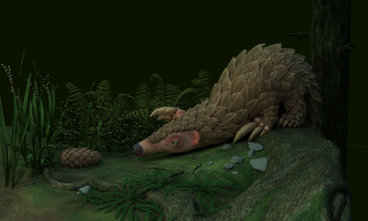
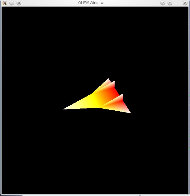
Notice that there are only two traditional lights (lamps). The arcade is mostly lit by indirect light, the cubes are shining from every point on the surface.

And I’m quite proud that I won the first place in the course’s contest :D

Now that you’ve seen the video, I’d like to talk a bit about the technology. In the end there is a conclusion, which you shouldn’t skip. Finally there is information on how to retrieve the code and executables.

Technology

I implemented a deferred rendering system using OpenGL and CUDA. The bouncing cubes are computed with Bullet by simply applying random forces. There are two main spot lights computed via shadow maps, indirect light is computed via ray tracing.

All geometry and texture information is rendered into a buffer on the GPU using OpenGL. The shadow maps are also rendered by OpenGL. Until here it is a standard deferred rendering system and therefore I’ll skip the details. Those buffers are then passed to CUDA, where the shading happens. This shading stage is divided into several CUDA kernels.

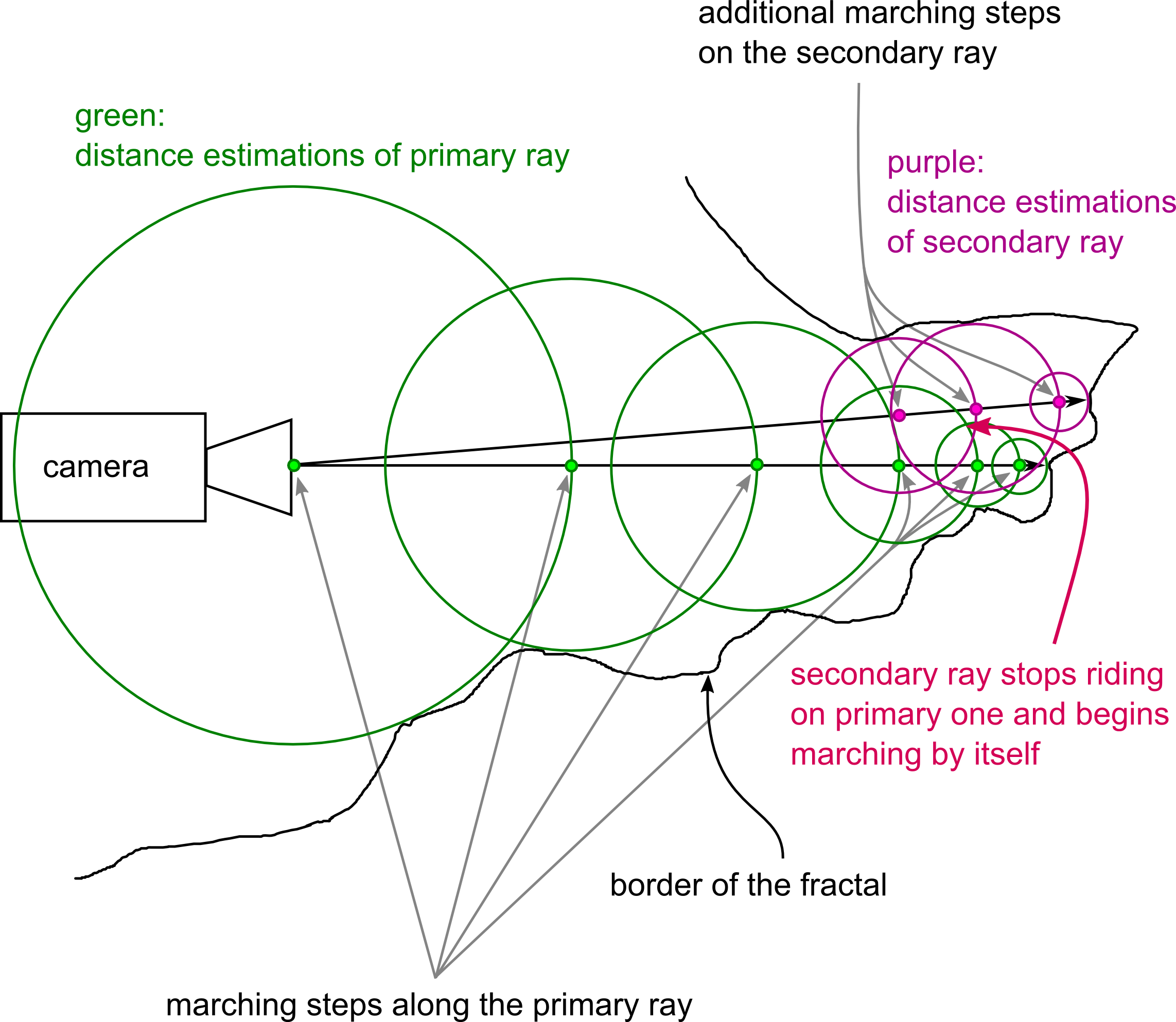
  • The first is doing the ray tracing.
    It is path tracing with only two bounces:
    camera —–> surface —–> surface —–> light.
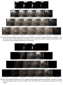
    The first ray from the camera is not computed and taken from the geometry buffer instead. The last ray isn’t computed as well and taken from the shadow map instead. So only the middle ray is traced. Since indirect light usually contains only low frequencies, it is possible to compute it only in half of the resolution with only very little quality impact and big performance gain. On the half resolution image, 2-16 rays are computed per pixel (in the download you’ll find several executables, the quality refers to the number of rays per pixel. If I remember correctly, 4 rays per pixel were used for the video, this runs in real time (>30fps) on a modern GPU). For ray tracing itself I adapted a highly optimised kernel developed by Finnish NVIDIA engineers, along with a good BVH builder from the same source.
  • The next kernel filters the result from the ray tracing kernel. This filter is blurring, but it takes normals and distance into account, so that indirect light doesn’t get blurred over edges. The filter is not separable into a horizontal and vertical pass, because of the additional information taken into account. There were bandwidth and latency issues with the kernel and so I had to put quite some effort into optimising it.
  • Finally there is the main shading kernel, which computes the traditional shading and adds the indirect light. This is quite strait forward, there is just a little catch. Since the indirect light is computed in a lower resolution, in some cases there where ugly aliasing effects. Imagine a dark polygon in the foreground and a bright, indirectly lit one in the background. This situation would result in 2×2 steps across the edge. This is alleviated by another blurring stage, which takes normals and distance from the higher resolution buffer into account. So on pixels on polygon edges, which would take the colour of the underlying 2×2 block from a different polygon before, now the filtering would only take the colour from the correct polygon.

After the CUDA part finished, the buffers are handed back to OpenGL for post-processing: basic tone mapping, bloom, lens flares. Since I based firefly on a previous project’s OpenGL engine, those effects were already implemented. I won’t go into details because the effects are pretty standard and there are already a lot of sources.

Conclusion

Ok, so usually one should write how cool it was and how good the method worked. I’m an honest person: It was cool to program, I learned really a lot, I won the first place, I don’t regret, but the approach is bad, don’t try it out :), here is why:

My university tutors feared that the switch between OpenGL and CUDA would be too expensive, but this was not the case. Naturally there are costs, but those are way under 1 ms (unpacking geometry data and writing the output in CUDA costs about 1 ms, which includes already some computation work, while ray tracing takes around 30 ms). So this was the positive side: you can switch between OpenGL and CUDA every frame, if you do it right, the performance will be OK.

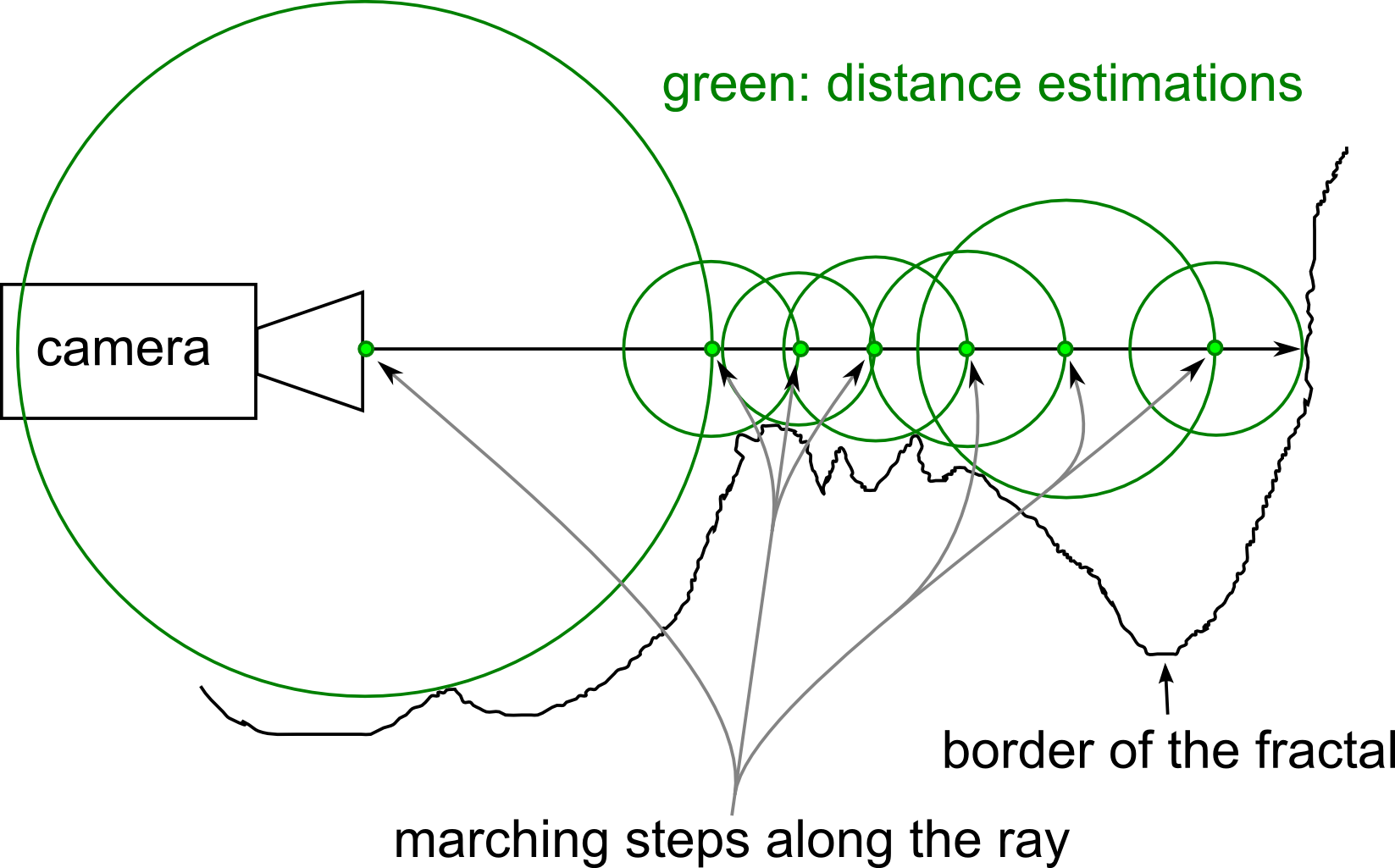
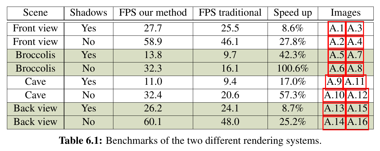
But to understand why the approach is only mediocre, one needs to understand how ray tracing performs on the GPU. Almost parallel rays are fast, random rays are slow. The reason is that “similar” rays will need mostly the same elements from the Bounding Volume Hierarchy, execution and data divergence will be low. Random rays are the opposite. That’s why it’s possible to get more than 60 fps when shooting only primary rays, while shooting just one random ray per pixel from the surface originally brought the performance to under 10 fps. Similarly it should be possible to compute rays from the lamps to the surface in a fast way, but it might include sorting and I didn’t test that.

So the approach from above accelerates the fast part of a 2 bounce path tracing algorithm, but the slow part – computing a random ray from one surface to another – stays slow.

It would be much better – from a software engineering perspective – not to mix ray tracing and the traditional pipeline in this case, because costs are to high compared to the benefits. A lot of data is duplicated on the graphics card, it is cumbersome to program, tradeoffs make performance okeyish, but quality is not great (look at the flickering and noise). It’s just not production ready and it will never be. It’s better to wait another couple of years until GPUs will be fast enough to do real path tracing in real-time.

While starting to program, I was also thinking of implementing caustics. Those could produce really nice effects and be over 60 fps – depending on the quality of the caustics, which could justify ray tracing. If somebody tries that, please let me know about it in the comments. In my case I couldn’t do it due to time constraints.

On a side note, I wasn’t thinking about NVIDIA OptiX due to past experiences with it. I was quite satisfied with CUDA, a ray tracing library would be cool, but that’s a pretty big wish : )

Code and Executable

You can use my old repository directly. The last version of the demo code is tagged, there are a few more revisions for another lecture’s submission.

I have packed everything together into a zip file. There are Windows and on Linux versions. You’ll need an NVIDIA graphics card and recent drivers. You might also need CUDA and you might need to delete the CUDA library files, it’s hard to deploy to unknown systems, do whatever works for you :) . I used CUDA 6.5..

Global illumination rendering using path tracing and bidirectional path tracing

This year I started a course on Advanced Computer Graphics in Aalto University by Jaakko Lehtinen. The focus was on methods for global illumination (GI). In a nutshell, global illumination means more realistic lighting compared to “traditional”, direct lighting, where light is reflected by all surfaces (including diffuse ones). Therefore the shading includes indirect light, colour bleeding, caustics etc. Think of a room with only one window and no additional light, the wall with the window will be also illuminated, but only by light that was reflected from the floor and other walls.

There are many methods of implementing GI, for instance photon mapping, instant radiosity, path tracing and bidirectional path tracing or the quite involved method of Metropolis light transport (MLT). It was obligatory to implement path tracing, but I implemented bidirectional path tracing in addition. As a bonus, I implemented both of the methods on the graphics card using the OptiX Framework from NVIDIA, but please don’t make the same mistake of using OptiX.

Path tracing

Path tracing means tracing a path from the camera, bouncing off of surfaces in a random direction, and doing so until the ray hits the light. On every bounce the reflectance function is used to calculate the amount of reflected light. For instance a red surface would reflect only red light, a white surface all of it and a black one nothing. Naturally one sample is not enough, several samples are taken per pixel and the average gives the actual colour. This results in an unbiased estimation of the colour at the pixel. The technical term for this is Monte Carlo integration.

There are many ways to speed up the convergence, I implemented the following (some of them reused for the bidirectional path tracer):

  • At every bounce one additional ray is shot into the direction of a light. This is especially important if the light source is small and hitting it randomly has a small probability. In order not to add the energy from the light twice, a random hit should be ignored.
  • The randomly reflected ray should not be sampled according to an uniform distribution, but to a distribution matching the reflectance function and a geometrical term (importance sampling). This gets even more important with a micro-facet model, which was used to simulate partly reflective surfaces (the same model was used for the normal path tracer and the bidirectional one).
  • Numbers from a random number generator tend to cluster, which is not optimal for Monte Carlo. A Low-discrepancy sequence is better, because the area of integration is covered more evenly. The Wikipedia Article about the Halton sequence shows the difference.

Bidirectional path tracing

Difference between bidirectional and normal path tracing (from Veach's PhD thesis).
Difference between bidirectional and normal path tracing (from Veach’s PhD thesis).

The idea of this method is quite simple, but the implementation is involved. Normal path tracing sometimes has difficulties to sample the light, especially when there are caustics or the light is a bit hidden as it is in the scene above. The reason in both cases is that it can’t be sampled directly (shooting a ray into the direction of the light) and hitting it randomly is improbable. More generally, normal path tracing has difficulties to sample important paths in certain situations, resulting in a noisy image.

Different bidirectional sampling techniques, taken from the Mitsuba documentation.

Bidirectional path tracing shoots rays from both directions, from the light and from the camera. This results in two paths consisting of vertices, the light and the eye/camera path. Then each camera vertex is connected to each of the light vertices, forming different paths for transporting light. Eric Veach calls them bidirectional sampling techniques. These techniques have different “fields of expertise”, meaning that certain techniques are only efficient for certain effects. The figure on the right shows a collection of such sampling techniques.

In order to compile them into an image, they are weighted and added up. Computing the weight is a bit complex, but basically it’s computing the probability of generating the specific path divided by the sum of generating any path with vertices at the same positions. This results in switching off the techniques for effects that they can’t sample efficiently and therefore results in an image with less noise. This can be observed in the bottom part of the figure on the top right. The technical term is multiple importance sampling and is also covered in depth in Veach’s thesis.

After implementing the base of the algorithm with perfectly diffuse surfaces, I also added perfectly refractive and reflective surfaces as well as micro facet type surfaces (math taken from here).

Sub Surface Scattering

Finally I also implemented sub surface scattering. This book contains an excellent explanation of it (the papers (1, 2) by Jensen et al. aren’t so good in my opinion). I chose the accelerated version of the algorithm. This means that I have an octree containing surface points of cached irradiance. It seemed like this is not so cool as expected, the cache needs a lot of space in memory and the objects are lacking the montecarlo noise, which makes them look a bit odd. Blender’s renderer, Cycles, also doesn’t use the acceleration structure, instead they sample the surface directly. If I ever have to implement SSS another time, I’ll do it the Blender way. But for this project I chose to use a hack: In order to fix the unusual look, I mixed in the normal diffuse reflection. So a SSS surface is now 50% SSS and 50% perfectly diffuse.

Results

Because I implemented so many features, I didn’t have enough time to choose nice scenes.

There is one Pangolin, based on a model made by my sister:

Rendering of a Pangolin
The body contains a term for SSS, it filled up the video memory almost completely: 96%.

then there is the famous Sponza:

Sponza, featuring a simple path tracer and diffuse surfaces

and finally a demo scene for the bidirectional tracer:

Bidirectional Test Scene
The glass was modeled by me, the rest are primitives from Blender. The scene features caustics, reflective and refractive surfaces, micro-facet model surfaces, some lights and diffuse surfaces.

Code

I was asked to provide the code. Since the project is based on the OptiX Samples framework and the framework has a proprietary license, I can’t give you the full project. Instead I made a diff to the sample directory provided with OptiX 3.0 (as this was the current version when I started coding).

To make it work you need:
1. download OptiX 3.0
2. apply the patch, under Linux it should be possible with the patch tool, something similar should exist on windows
3. if you want to compile and execute my code, download and compile Assimp and FreeImage (the dll’s and header files are assumed to be in folders next to the project folder)
4. follow the instructions in the readme file.

If you have any questions or problems with compiling, feel free to contact me. Preferable via the answer function, so others can also benefit..

Here is the patch.

Real Time 3d Mandelbulb

Render of a 3d Mandelbulb

It’s actually already almost one year since I finished the work on an Erasmus project in Universitat Politècnica de València, Spain. The goal was to speed up the computation of distance estimated 3d fractals in a way so that they could be computed in real time and therefore make it possible to explore them in an interactive fly through program.

Fractals are graphics produced by recursive mathematical formulas. Sine the graphics are purely based on math, one can zoom in infinitely into them without loosing quality, well – as long as the float precision is enough. One classical 2d fractal is the Mandelbrot. Some years ago a formula for a 3d Fractal was found that resembles a Mandelbrot and the structure was called Mandelbulb.

Although there already exist programs that do the fractal computation on the graphics card, none of the ones I found was able to do it in acceptable quality and real time. Some of them produced nicer images, but at the cost of having long rendering times, others where sort of interactive, but the quality was bad.

I first implemented a quick proof of concept using NVIDIA OptiX, based on their Julia example, but OptiX quickly showed its limitations, especially when I started to work on a method to speed the thing up. So I switched to NVIDIA CUDA and was satisfied with that decision (and anyway, as I will blog soon, I recommend to stay away from OptiX as far as possible : ).


I’ll explain in a few sentences how the rendering works, details for the traditional method can be found on the page of Mikael Hvidtfeldt Christensen and for both, the traditional and improved one  in my report linked below.

Figure explaining ray marching
ray marching

There is a function, which returns the maximum lower bound for the distance to the fractal, called the distance estimator (DE). When walking along a ray, for instance shot by the camera, it is safe to walk this distance, because we have the guarantee that the fractal won’t intersect the ray in this interval. After one step, the distance is estimated again and we march as long, as the estimated distance is above a certain threshold.

My idea to speed up the rendering was to decrease the amount of computation by letting neighbouring rays “ride” on the previous rays.

Principle of the new algorithm

This works in two passes, first, “primary” rays are shot with a distance of several pixels to each other, recording the DE values. Secondly, the neighbours, called secondary rays in the figure, are shot. Those can use the information calculated in the first pass to jump straight to the end of the stepping. So, that’s it, in short. Don’t confuse the terms primary and secondary rays with bouncing light of ray tracing here.

Benchmarks of the new algorithm compared to the old one from the report

Comparing the traditional ray marching algorithm with the new, faster one, shows a speed up of up to 100% and interactive exploration in almost all views without shadows. It would be probably possible to also implement this speed up for shadow rays, but I had no time to do it. Unfortunately there are some artefacts due to the ray “riding”, details can be found in the report. If you are interested into the source code, please write me a message.

Edit: The  reason I don’t publish the repository is that there is still some (c) NVIDIA code inside (setting up CUDA, the render window etc). If there is somebody willing to replace / redo that code with something GPLv3, check the build and maybe update to the newest sdk, that would be most welcome :)

Edit2: Ok, the GPL parts of the source code are published now. I’m aware that it does not compile, however I haven’t got the time to replace the NVidia parts taken from the examples. Maybe it’ll help some of you anyways :)

Merging Ray Tracing and Rasterization in Mixed Reality

Reflection Scene rendered by our combined renderer

I’ve been studying computer sciences for three years and recently I finished writing my bachelor thesis. The topic was implementing reflections and refractions in the context of mixed reality. Basically, mixed reality means adding virtual objects into a video stream (of real environment). One of the goals is to make the resulting images look as realistic as possible. Naturally this includes reflection and refraction effects.

In my work I utilise the framework implemented in the RESHADE project. There was already a mixed reality renderer based on a Direct3D rasterizer. My task was to work on a ray tracer using OptiX and merge the resulting image with the rasterizer’s image. OptiX provides a ray tracing framework for the graphics card.

Glass Bunny Scene
Glass Bunny Scene

Generally a ray tracer is slower than a rasterizer, but it has better quality with reflections and refractions. Because of that, we used a combined method. The ray tracer is working only on transparent and reflecting surfaces. This is achieved by a mask, which is created by the rasterizer in a separate render pass. This mask indicates, where reflecting or refracting objects are.

Especially with virtual flat mirrors there are very strong artefacts (see reflection scene, right mirror). This is due to lack of information. We are using the video frame, the environment map and the textured model of the real scene to gather information for the reflected ray.

Other problems we encountered were artefacts due to different shading algorithms in the rasterizer and ray tracer, and various issues with implementation due to the tone mapper.

When I was more or less finished with my work, I discovered that somebody else in the project was working on the implementation of reflections and refractions using the rasterizer. This was cool, because we were able to compare the results. Usually rasterizing is much faster than ray tracing. Surprisingly this was not the case with all scenarios. The reflection scene (first image) was faster with the combined method, the transparent bunny was slower. Especially with the bunny scene, I believe that the main drawback in speed was accuracy. The ray tracer also computes inner reflections, which causes a lot of additional work. I didn’t manage to benchmark this (rendering without inner reflections), because I was running out of time, but maybe I will do it yet..

Thanks to Michael Wimmer for making this work possible and special thanks to Martin Knecht for being an excellent supervisor and helping with all the questions :).

Finally, if you are interested into more details, here you can find the thesis..

Chawah, Final update a little latish..

I had lots of things to do, no time etc etc. You know the excuses. But now I want to write another blog about a new Lindenmayer brush for Krita, and though have the motivation to catch up with old posts..

Well, we added loads of new features, mainly graphical ones:

  • lens  flares and sun dazzle effect
  • moving space dust (white circles), which are moving randomly, this is an simple particle system.
  • explosion and fire stream effects (more complicated particle systems)
  • environment mapping (on the ships and station)
  • bloom
  • music and sound effects
  • some power ups (armor, rockets, boost)

Here is the video that we made for the presentation.

Chawah Progress

More than one month since my last post and we (Felix and me) are quite satisfied with our progress. There is some basic game logic (you can destroy the other ship and then the game restarts), health display and physics. We got all points at our first submission and currently we are starting implementing the effects. Environment mapping is already in place.

I’ve made a short video, where you can see bullet physics in action (at the end of the video you can see bullet debug mode enabled).

First chawah screenshots

Unfortunatly I hadn’t time for Krita any time recently. I had to work and do stuff for university. I will focus more on Krita in summer again..

This term i’m attending the second computer graphics course in my university. The goal is to program a 3d game in OpenGL. We (Felix and me) chose to program a split screen flight duel game, as this is a simple game concept, but it’s still very extensible graphics and game logic wise.

The first step was to setup OpenGL etc. (GLEW, GLFW), which produced this first screen shot in begin of April.
First Chawah screen shot

We have worked hard and now we have implemented model loading (Assimp), shading, texturing, controls and split screen. Looks good for our first deadline :)
First Chawah screen shot

Next steps will be to implement some more game logic, in game display of hull state, frags and menu and then physics. We will use CEGUI and Bullet for these tasks..